Calculating Connectivity Rank for Bike Network Planning

You've got a plan to build out a 100 miles of of additional bike facilities. Which ones should you build first to make the biggest impact?

In addition to all the metrics that would usually apply to bike lane planning, now there are a few others that are interesting to consider in the priority: Does a segment fill in a gap in the existing network? Does it connect with the existing network? Is it a smaller, cheaper segment to complete?

Minneapolis has exactly this situation. To quantify and map the answer to these questions, I calculated a "Connectivity Rank" metric for every new segment of their near-term low-stress planned bike network.

The algorithm considers two elements to generate the rank:

1. How far is the segment from the existing bike network, where the distance is calculated using biking time from the segment to the existing network, following exclusively routes on the current and planned bike network. Notably, it does not factor in bike directions would require being on busy streets.
2. How long is the segment? Shorter segments are cheaper to build and rank better.

Here you can see what the result looks like. Below I'll explain the method.

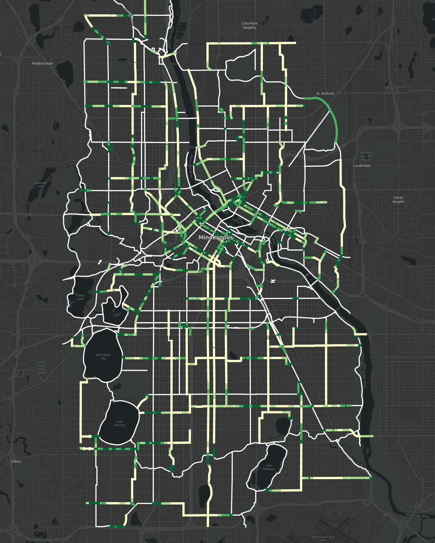
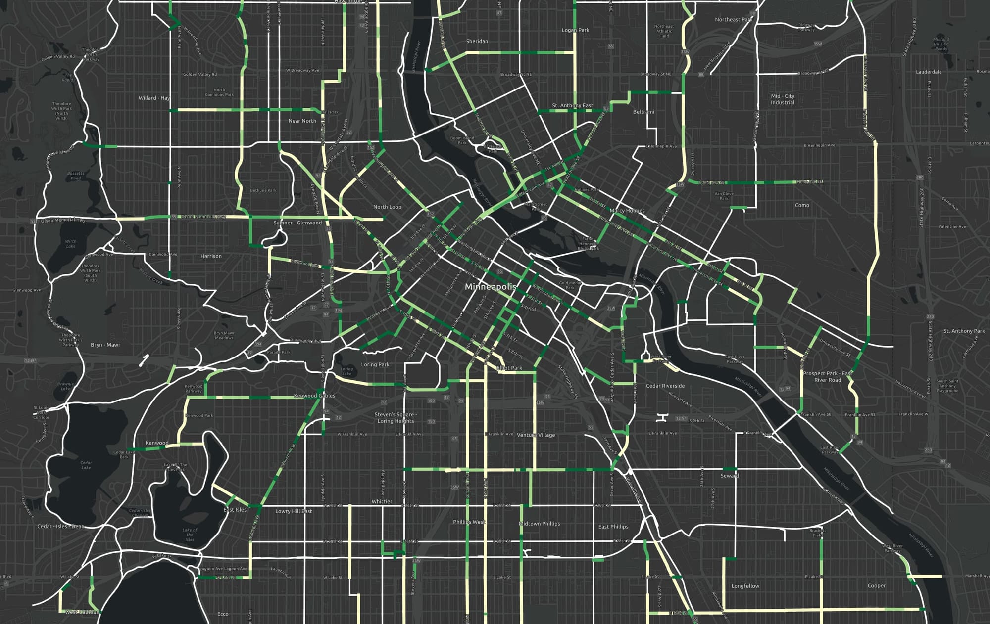
Here's a close-up of the city center:

How connectivity rank is determined

The first step for this was to generate 1, 2, 3, 4 and 5 minute bike-time isochrones from the existing network. For that, I used Valhalla for routing, which has a default bike speed of 11.5 MPH (18 KPH).

Normally, bike-time isochrones are generated using the entire routable road network-- busy streets and everything.

First, I needed the current and future bike network in the ".osm.pbf" format understood by Valhalla, without the rest of the road network.

To do that, a few conversions were required. Starting with GIS data for the bike network, I:

1. imported into QGIS
2. filtered to just the bike network.
3. exported the result to GeoJSON
4. Imported into JOSM
5. Add OSM-recognized tags so the network would be routable. I used highway=residential and bicycle=designated. The exact tags don't matter so long as Valhalla recognizes them as valid for bicycle routing.
6. Save the result in .osm.pbf format
7. Launch Valhalla from the directory containing the .osm.pbf file:

docker run --rm  --name valhalla -p 8002:8002 -v $PWD:/custom_files ghcr.io/gis-ops/docker-valhalla/valhalla:latest

And with that, I have a customized isochrone web server running on port 8002 on my laptop.

From there, I generated the isochrones using the custom Node.js code in low-stress-network-analysis.mjs.

That uses as an input a hex grid for the city. ArcGIS and QGIS can generate such grids. I have a Node.js script to generate the hex grid for a city when given it's boundary. I use a cell side length of 0.05 km.

This script finds all the places where the existing network intersects with the hex grid, and generates isochrones from the center of all those hex grid cells. Then, it joins all the isochrones together into one giant isochrone for the entire network for "1 minute from the existing network by bike". It then repeats the process for 2, 3, 4, and 5 minutes by bike. For Minneapolis, it generated and merged something like 17,000 isochrones down to the 5. Seems like the whole process took about 30 minutes to run on my laptop, although I didn't actually time it.

That brings us to the steps completed by the second script add-connectivityRank-to-near-term-network.mjs.

This one uses the "near term" network, the hex grid and the five isochrones to iterate through the entire near-term network segments again, considering the segments at the scale of the size of hex cells. For each hex-cell size bits, it checks to see if the location is 1, 2, 3, 4 or 5 minutes from the existing network and increments the connectivity rank. Longer segments that have ranks that go to 50 or higher. In this way, shorter segments and segments closer to the existing network both rank higher. If a segment is short AND close the existing network, even better.

The final product is a file named near-term-with-connectivity-rank.geojson. It is the sameis the near-term network file provided as input, but with a connectivityRank property added to each segment. Lower ranks are better.

A zero rank means "no rank" and are not useful. That occurs in a few places for facilities that that technically outside the city limits and not covered by the hex grid. To consider faciltiies that extend beyond the city limits, use a larger hex grid.

For ideas on how to combine this metric with others for a more complex priority calculation, see the method described in Sidewalk Priority Map.